“Historically what’s happened is, when there’s a spike [in inflation], the spike persists for a long time. Inflation tends to be highly persistent once you get it.”
Eugene Fama
Nobel Prize Economics, 2013
Distinguished Professor of Finance
University of Chicago
“There is no way of slowing down inflation that will not involve a transitory increase in unemployment, and a transitory reduction in the rate of growth of output. But these costs will be far less than the costs that will be incurred by permitting the disease of inflation to rage unchecked.”
Milton Friedman
Nobel Prize Economics, 1976
Former Professor of Economic Theory
University of Chicago
“Part of the problem is the Fed has gotten involved in a multitude of ways in the financial market. There’s only so much central banks can do. And when they claim they can do more than that, they tend to get into areas where they should not be.”
Raghuram Rajan
Former Governor of Reserve Bank of India
Distinguished Professor of Finance
University of Chicago
Market Review
Below are some of the indices we track. It has been a really tough environment since January 1.
| Data Series | YTD | 3 Months | 6 Months | 1 Year | 3 Years | 5 Years | 10 Years |
| Russell 3000 | -24.62% | -4.46% | -20.42% | -17.63% | 7.70% | 8.62% | 11.39% |
| S&P 500 | -23.87% | -4.88% | -20.20% | -15.47% | 8.16% | 9.24% | 11.70% |
| Russell 2000 | -25.10% | -2.19% | -19.01% | -23.50% | 4.29% | 3.55% | 8.55% |
| Russell 2000 Value | -21.12% | -4.61% | -19.18% | -17.69% | 4.72% | 2.87% | 7.94% |
| MSCI World ex USA | –26.23% | -9.20% | -22.50% | -23.91% | -1.21% | –0.39% | 3.62% |
| MSCI World ex USA Small Cap | -31.07% | -9.46% | -25.70% | -30.80% | -1.27% | -1.24% | 4.78% |
| MSCI Emerging Markets | -27.16% | -11.57% | -21.70% | -28.11% | -2.07% | -1.81% | 1.05% |
| Bloomberg U.S. T Bond 1-5 Yrs | -6.35% | -2.25% | -3.09% | -7.05% | -1.04% | 0.35% | 0.59% |
| ICE BofA 1-Year US T Note | -1.77% | -0.50% | -0.97% | -1.95% | 0.18% | 0.94% | 0.67% |
There has been nowhere to hide, although short-term high-quality bonds, as evidenced by the last 2 rows of the returns above, have tempered the larger downturns of the stock market. What is going on?
Inflation
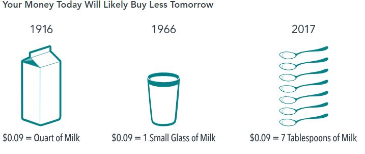
In this newsletter, we are going to focus on inflation and its impact on the markets. As Professor Nicholas Li states, “inflation refers to a general increase in prices and the resulting decline in the purchasing power of money.” When the prices of goods and services increase over time, consumers can buy fewer of them with every dollar they have saved. Therefore, keeping pace with inflation is an important goal for investors. When the rate of increase is larger and faster, the resulting decline in purchasing power is more painful. Below is a graphic explaining how money today buys less tomorrow.

In US dollars. Source for 1916 and 1966: Historical Statistics of the United States, Colonial Times to 1970/US Department of Commerce. Source for 2017: US Department of Labor, Bureau of Labor Statistics, Economic Statistics, Consumer Price Index—US City Average Price Data.
We have become somewhat spoiled over the past 20 years, as inflation has remained subdued prior to late 2021. However, concerns have been building for a while. In my newsletters sent on June 12, 2020, and July 12, 2021, I expressed concern about the rapid rise in the money supply in the United States, as evidenced by what is known as M2. I tried to explain what economist Milton Friedman stated years ago:
“Economist Milton Friedman was quoted as saying “inflation is taxation without legislation.” Thinking of inflation as a tax is useful because the reality is that inflation erodes your purchasing power. Said differently, $1 was able to buy more things in 1947 than it can buy today. Figure 2 shows how the purchasing power of $1 in 1947—the longest history available at the BLS website—has declined through time. Today, that same dollar buys about 8 cents’ worth of goods.”
Friedman stated that inflation “is always and everywhere a monetary phenomenon in the sense that it is and can be produced only by a more rapid increase in the quantity of money than in output.” Or as Professor Aswath Damodaran of NYU states in his May 24,2021 blog post, “too much money chasing too few goods.” Professor John Cochrane wrote in May, “where did inflation come from, is question number one, and Charlie Plosser gave away the answer in his nice preface to this session: The government basically did a fiscal helicopter drop, five to six trillion dollars of money sent in a particularly powerful way. They sent people checks, half of it new reserves, half of it borrowed. It’s a fiscal helicopter drop.” Hence, a “more rapid increase in the quantity of money than in output.”

Tyler Cowen, professor of economics at George Mason University, recently wrote:
“Consider the recent spurt of 8% to 9% inflation in the US. The simple fact is that M2 — one broad measure of the money supply — went up about 40% between February 2020 and February 2022. In the quantity theory approach, that would be reason to expect additional inflation, and of course that is exactly what happened.
The quantity theory has never held exactly, one reason being that the velocity (or rate of turnover) of money can vary as well. Early on in the pandemic, spending on many services was difficult or even dangerous, and so savings skyrocketed. Yet those days did not last, and when the new money supply increase was unleashed on the US economy, there were inflationary consequences.”
In addition to the monetary phenomenon, additional supply shocks have occurred due to both Covid in 2020 and the Russian invasion of Ukraine. As Cochrane eloquently states, “while supply shocks can raise the price of one thing relative to others, they do not raise all prices and wages together.”
How does the Federal Reserve slow inflation? According to Friedman by an increase in unemployment, and a reduction in the rate of growth of output. One way the Federal Reserve does this is by raising the Federal Funds Rate, which is the target rate at which commercial banks borrow and lend their excess reserves to each other overnight. That rate, which is considered the “risk free” rate, influences other short-term rates.
In the short term, a rapid rise in the risk-free rate, all else being equal, will cause asset prices to adjust downward because stocks are essentially valued by discounting their estimated future cash flows by an interest rate. The rate includes both the “risk free rate” that the Federal reserve is raising as well as a risk component, which can be described as the “equity risk premium,” which is also rising.
According to Damodaran in his September 26, 2022, blogpost:
“There are two things that stand out about equity markets in 2022. The first is the surge in the equity risk premium from 4.24% on January 1, 2022, to 6.05%, on September 23, 2022, an increase on par with what we have seen during market crises (2001, 2008 and 2020) in the past. The second is that as equity risk premiums have jumped, the treasury bond rate has more than doubled, from 1.51% on January 1, 2022, to 3.69% on September 23, 2022. In contrast to the afore-mentioned crises, where the treasury bond rate dropped, offsetting some of the impact of the rise in equity risk premiums, this inflation-induced market reaction has caused the expected return on stocks to rise from 5.75% on January 1, 2022, to 9.75%, on September 23, 2022; that increase of 4% dwarfs the increases in expected returns that we witnessed in the last quarter of 2008 or the first quarter of 2020.”
The good news is that expected returns going forward are greater than they were in January. Professor Fama advises not to get out of the market now, because “if you bounce in and out of the market in response to variation in volatility, you are likely to be in when expected returns are low and out when expected returns are high.” Since expected returns are higher now, an investor would want to stay in the market to try and capture those expected returns. It does not mean that we will not experience volatility. As uncertainty lingers, so will volatility. Predicting volatility is virtually impossible. Fama states “bouncing in and out only makes sense if you can forecast increases and decreases in volatility before they occur, so you can miss the price declines associated with the onset of high volatility and profit from the increases associated with the onset of low profitability. I doubt that anyone is that good at predicting changes in volatility.”
Unless one can predict the future increases and decreases in volatility and price, the better approach is to have an asset allocation that one can stick with during good times and bad. As our friends at Dimensional have written, “inflation is an important consideration for many long-term investors. By combining the right mix of growth and risk management assets, investors may be able to blunt the effects of inflation and grow their wealth over time. Remember, however, that inflation is only one consideration among many that investors must contend with when building a portfolio for the future. The right mix of assets for any investor will depend upon that investor’s unique goals and needs.”
David Berns, author of Modern Asset Allocation for Wealth Management and co-founder of Simplify, takes a consistent approach to Dimensional and Fama above by stating that “a slightly lower utility portfolio adhered to is better than a portfolio with higher utility that is not adhered to, if your goals can handle such accommodation.” His thoughts are consistent with Fama advising not to get out of the market, as timing is virtually impossible to be right on getting back in the market again, especially on a consistent and persistent basis. It is most likely better to be invested in a more conservative portfolio (which is less volatile) that you can stick with versus an aggressive one (which is highly volatile) that you cannot.
Our friends at Avantis Investors have written recently:
“What stands out is that the below-average returns we’ve seen historically during times of recession have been driven by significantly negative returns during the first half of the recession. In the second half of recessions, returns have been strongly positive and far above the average monthly return. Good times have historically continued during the first and second halves of expansions…
It would be great if we could get out of the market at the start of a recession before stocks typically experience a downturn and then get back in as prices go back up. The issue is that we can’t say with certainty when economic peaks and troughs will start and end until after the fact — and trying to time these events can have detrimental effects on investors if they get it wrong.
Considering where we are today, we’ve already seen U.S. stocks decline significantly. We can’t know for sure, but it may be that we are currently experiencing the disappointing returns often seen during the first half of recessions. The market seems to have already priced in a lot of bad news and the potential for turmoil. The risk of fleeing the market today is that investors may leave when the bad news is priced in and miss out on the historically positive returns typically seen in the second half of recessions.”
We hope the above helps understand a bit more about what is going on. There are many different factors impacting the markets. Inflation is one factor.
The Real Thing
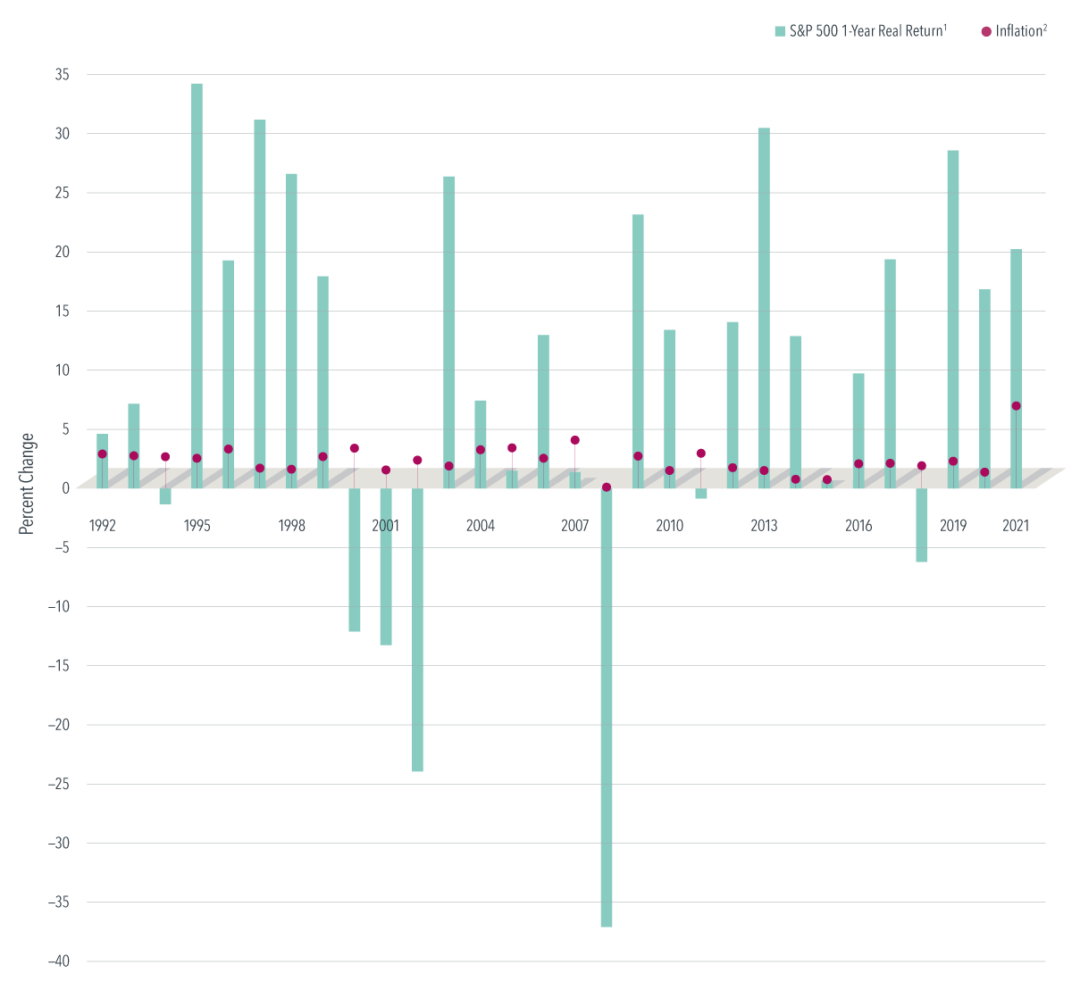
Annual inflation-adjusted returns of S&P 500 Index vs. inflation, 1992–2021

Past performance is no guarantee of future results. Indices are not available for direct investment; therefore, their performance does not reflect the expenses associated with the management of an actual portfolio. Copyright 2022 S&P Dow Jones Indices LLC, a division of S&P Global. All rights reserved.
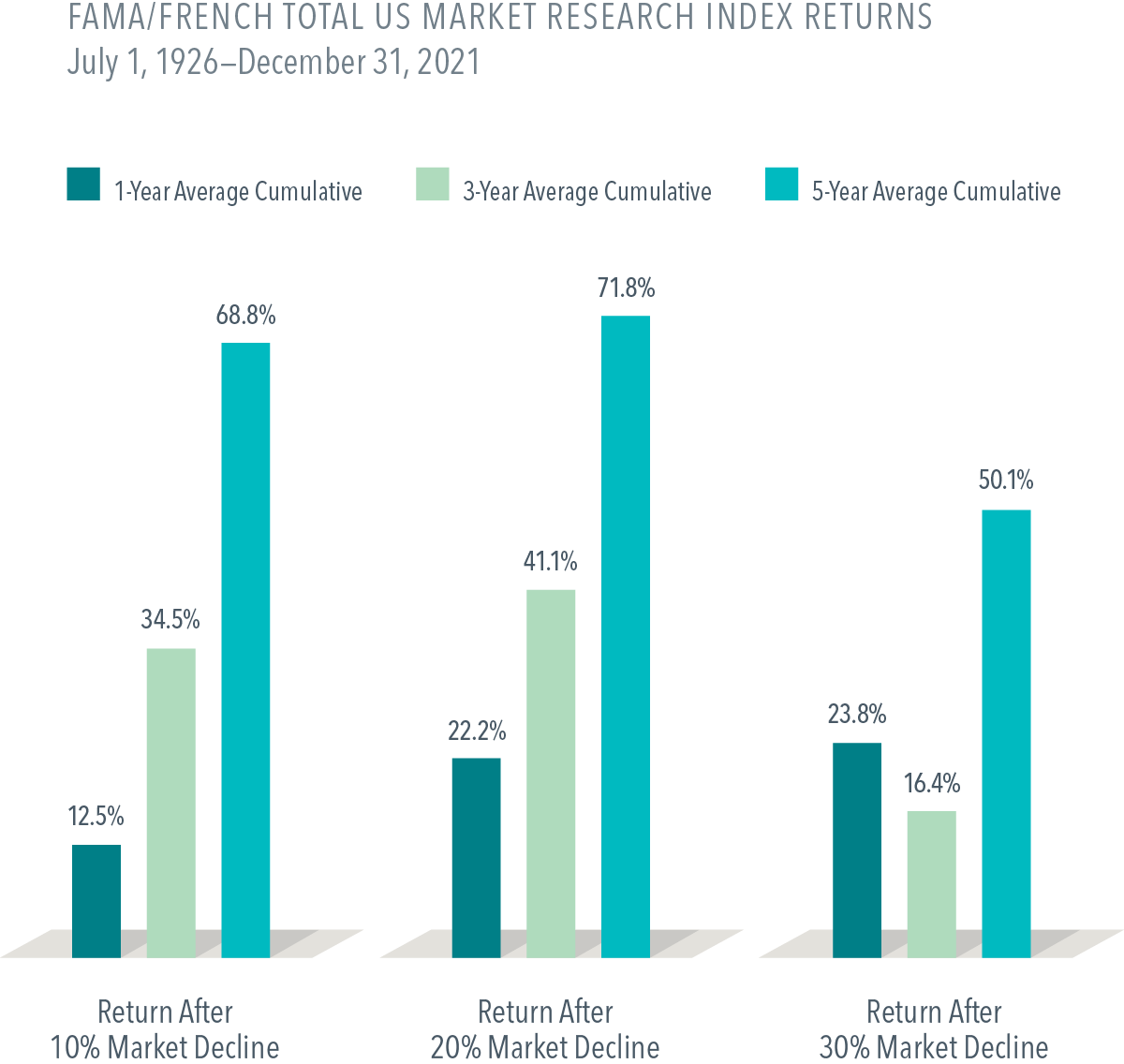
History shows that stocks tend to outpace inflation over the long term—a valuable reminder for investors concerned that today’s rising prices will make it harder to reach their financial goals. And one last chart on market rebounds.

Please don’t hesitate to reach out with any questions.
Until next time,
Emily and Mike
*Market declines or downturns are defined as periods in which the cumulative return from a peak is -10%, -20%, or -30% or lower. Returns are calculated for the 1-, 3-, and 5-year look-ahead periods beginning the day after the respective downturn thresholds of -10%, -20%, or -30% are exceeded. The bar chart shows the average returns for the 1-, 3-, and 5-year periods following the 10%, 20%, and 30% thresholds. For the 10% threshold, there are 29 observations for 1-year look-ahead, 28 observations for 3-year look-ahead, and 27 observations for 5-year look-ahead. For the 20% threshold, there are 15 observations for 1-year look-ahead, 14 observations for 3-year look-ahead, and 13 observations for 5-year look-ahead. For the 30% threshold, there are 7 observations for 1-year look-ahead, 6 observations for 3-year look-ahead, and 6 observations for 5-year look-ahead. Peak is a new all-time high prior to a downturn. Data provided by Fama/French and available at mba.tuck.dartmouth.edu/pages/faculty/ken.french/data_library.html. Fama/French Total US Market Research Index: 1926–present: Fama/French Total US Market Research Factor and One-Month US Treasury Bills. Source: Ken French website.

